Display Time-Domain Data
The following tutorial shows you how to configure the Time Scope blocks in the ex_timescope_tut model to
display time-domain signals.
Open the Time Scope Model
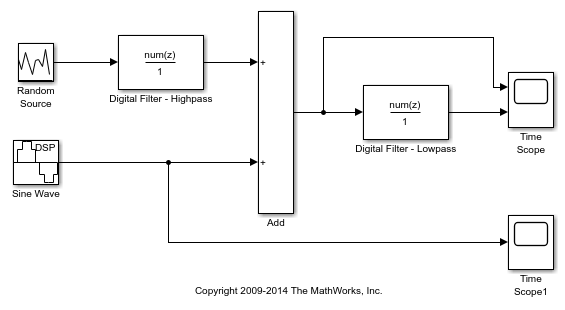
To get started with this tutorial, open the ex_timescope_tut model.
Use these workflows to configure the Time Scope blocks in the ex_timescope_tut model.
Configure the Time Scope Properties
The Configuration Properties dialog box provides a central location from which you
can change the appearance and behavior of the Time Scope block. To open the
Configuration Properties dialog box, you must first open the Time Scope window by
double-clicking the Time Scope block in your model. When the window opens, select View > Configuration Properties. Alternatively, in the Time Scope toolbar, click the Configuration
Properties ![]() button.
button.
The Configuration Properties dialog box has four different tabs, Main, Time, Display, and Logging, each of which offers you a different set of options. For more information about the options available on each of the tabs, see the Time Scope block reference page.
Note
As you progress through this workflow, notice the blue question mark icon
(![]() ) in the lower-left corner of the subsequent
dialog boxes. This icon indicates that context-sensitive help is available. You
can get more information about any of the parameters on the dialog box by
right-clicking the parameter name and selecting What's
This?
) in the lower-left corner of the subsequent
dialog boxes. This icon indicates that context-sensitive help is available. You
can get more information about any of the parameters on the dialog box by
right-clicking the parameter name and selecting What's
This?
Configure Appearance and Specify Signal Interpretation
First, you configure the appearance of the Time Scope window and specify how the Time Scope block should interpret input signals. In the Configuration Properties dialog box, click the Main tab. Choose the appropriate parameter settings for the Main tab, as shown in the following table.
| Parameter | Setting |
|---|---|
| Open at simulation start | Checked |
| Number of input ports | 2 |
| Input processing | Columns as channels (frame
based) |
| Maximize axes | Auto |
| Axes scaling | Manual |
In this tutorial, you want the block to treat the input signal as frame-based,
so you must set the Input processing parameter to
Columns as channels (frame based).
Configure Axes Scaling and Data Alignment
The Main tab also allows you to control when and how Time Scope scales the axes. These options also control how Time Scope aligns your data with respect to the axes. Click the link labeled Configure... to the right of the Axes scaling parameter to see additional options for axes scaling. After you click this button, the label changes to Hide... and new parameters appear. The following table describes these additional options.
| Parameter | Description |
|---|---|
| Axes scaling | Specify when the scope automatically scales the axes. You can select one of the following options:
By default, this property is set to
|
| Scale axes limits at stop | Select this check box to scale the axes when the simulation stops. The y-axis is always scaled. The x-axis limits are only scaled if you also select the Scale X-axis limits check box. |
| Data range (%) | Allows you to specify how much white space surrounds
your signal in the Time Scope window. You can specify a
value for both the y- and
x-axis. The higher the value you
enter for the y-axis Data range
(%), the tighter the
y-axis range is with respect to the
minimum and maximum values in your signal. For example, to
have your signal cover the entire y-axis
range when the block scales the axes, set this value to
|
| Align | Allows you to specify where the block should align your data with respect to each axis. You can choose to have your data aligned with the top, bottom, or center of the y-axis. Additionally, if you select the Autoscale X-axis limits check box, you can choose to have your data aligned with the right, left, or center of the x-axis. |
Set the parameters to the values shown in the following table.
| Parameter | Setting |
|---|---|
| Axes scaling | Manual |
| Scale axes limits at stop | Checked |
| Data range (%) | 80 |
| Align | Center |
| Autoscale X-axis limits | Unchecked |
Set Time Domain Properties
In the Configuration Properties dialog box, click the Time tab. Set the parameters to the values shown in the following table.
| Parameter | Setting |
|---|---|
| Time span | One frame period |
| Time span overrun action | Wrap |
| Time units | Metric (based on Time
Span) |
| Time display offset | 0 |
| Time-axis labels | All |
| Show time-axis label | Checked |
The Time span parameter allows you to enter a numeric
value, a variable that evaluates to a numeric value, or select the
One frame period menu option. You can also select the
Auto menu option; in this mode, Time Scope
automatically calculates the appropriate value for time span from the difference
between the simulation Start time (Simulink) and Stop time (Simulink) parameters. The
actual range of values that the block displays on the time axis depends on the
value of both the Time span and Time display
offset parameters.
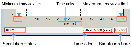
If the Time display offset parameter is a scalar, the value of the minimum time-axis limit is equal to the Time display offset. In addition, the value of the maximum time-axis limit is equal to the sum of the Time display offset parameter and the Time span parameter. For information on the other parameters in the Time Scope window, see the Time Scope reference page.
In this tutorial, the values on the time-axis range from
0 to One frame period, where
One frame period is 0.05 seconds
(50 ms).
Set Display Properties
In the Configuration Properties dialog box, click the Display tab. Set the parameters to the values shown in the following table.
| Parameter | Setting |
|---|---|
| Active display | 1 |
| Title | |
| Show legend | Checked |
| Show grid | Checked |
| Plot signal(s) as magnitude and phase | Unchecked |
| Y-limits (Minimum) | -2.5 |
| Y-limits (Maximum) | 2.5 |
| Y-label | Amplitude |
Set Logging Properties
In the Configuration Properties dialog box, click the Logging tab. Set Log data to workspace to unchecked.
Click OK to save your changes and close the Configuration Properties dialog box.
Note
If you have not already done so, repeat all of these procedures for the
Time Scope1 block (except leave the Number of input
ports on the Main tab as
1) before continuing with the other sections of this
tutorial.
Use the Simulation Controls
One advantage to using the Time Scope block in your models is that you can control model simulation directly from the Time Scope window. The buttons on the Simulation Toolbar of the Time Scope window allow you to play, pause, stop, and take steps forward or backward through model simulation. Alternatively, there are several keyboard shortcuts you can use to control model simulation when the Time Scope is your active window.
You can access a list of keyboard shortcuts for the Time Scope by selecting Help > Keyboard Command Help. The following procedure introduces you to these features.
If the Time Scope window is not open, double-click the block icon in the
ex_timescope_tutmodel. Start model simulation. In the Time Scope window, on the Simulation Toolbar, click the Run button ( ) on the Simulation Toolbar. You can also
use one of the following keyboard shortcuts:
) on the Simulation Toolbar. You can also
use one of the following keyboard shortcuts: Ctrl+T
P
Space
While the simulation is running and the Time Scope is your active window, pause the simulation. Use either of the following keyboard shortcuts:
P
Space
Alternatively, you can pause the simulation in one of two ways:
In the Time Scope window, on the Simulation Toolbar, click the Pause button (
 ).
).From the Time Scope menu, select Simulation > Pause.
With the model simulation still paused, advance the simulation by a single time step. To do so, in the Time Scope window, on the Simulation Toolbar, click the Next Step button (
 ).
).Next, try using keyboard shortcuts to achieve the same result. Press the Page Down key to advance the simulation by a single time step.
Resume model simulation using any of the following methods:
From the Time Scope menu, select Simulation > Continue.
In the Time Scope window, on the Simulation Toolbar, click the Continue button (
). Use a keyboard shortcut, such as P or Space.
Modify the Time Scope Display
You can control the appearance of the Time Scope window using options from the display or from the View menu. Among other capabilities, these options allow you to:
Control the display of the legend
Edit the line properties of your signals
Show or hide the available toolbars
Change Signal Names in the Legend
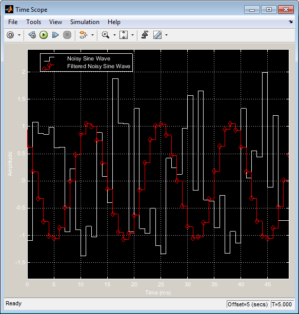
You can change the name of a signal by double-clicking the signal name in the legend. By default, the Time Scope names the signals based on the block they are coming from. For this example, set the signal names as shown in the following table.
| Block Name | Original Signal Name | New Signal Name |
|---|---|---|
| Time Scope | Add | Noisy Sine Wave |
| Time Scope | Digital Filter – Lowpass | Filtered Noisy Sine Wave |
| Time Scope1 | Sine Wave | Original Sine Wave |
Modify Axes Colors and Line Properties
Use the Style dialog box to modify the appearance of the axes and the lines for each of the signals in your model. In the Time Scope menu, select View > Style.
![]()
Change the Plot Type parameter to
Autofor each Time Scope block. This setting ensures that Time Scope displays a line graph if the signal is continuous and a stairstep graph if the signal is discrete.Change the Axes colors parameters for each Time Scope block. Leave the axes background color as black and set the ticks, labels, and grid colors to white.
Set the Properties for line parameter to the name of the signal for which you would like to modify the line properties. Set the line properties for each signal according to the values shown in the following table.
Block Name Signal Name Line Line Width Marker Color Time Scope Noisy Sine Wave ———— 0.5 noneWhite Time Scope Filtered Noisy Sine Wave ———— 0.5 
Red Time Scope1 Original Sine Wave ———— 0.5 
Yellow
Show and Hide Time Scope Toolbars
You can also use the options on the View menu to show or hide toolbars on the Time Scope window. For example:
To hide the simulation controls, select View > Toolbar. Doing so removes the simulation toolbar from the Time Scope window and also removes the check mark from next to the Toolbar option in the View menu.
You can choose to show the simulation toolbar again at any time by selecting View > Toolbar.
Verify that all toolbars are visible before moving to the next section of this tutorial.
Inspect Your Data (Scaling the Axes and Zooming)
Time Scope has plot navigation tools that allow you to scale the axes and zoom in or out on the Time Scope window. The axes scaling tools allow you to specify when and how often the Time Scope scales the axes.
So far in this tutorial, you have configured the Time Scope block for manual axes scaling. Use one of the following options to manually scale the axes:
From the Time Scope menu, select Tools > Scale Axes Limits.
Press the Scale Axes Limits toolbar button (
 ).
).With the Time Scope as your active window, press Ctrl + A.
Adjust White Space Around the Signal
You can control how much space surrounds your signal and where your signal appears in relation to the axes. To adjust the amount of space surrounding your signal and realign it with the axes, you must first open the Tools—Plot Navigation Properties dialog box. From the Time Scope menu, select Tools > Axes Scaling Properties .
In the Tools:Plot Navigation options dialog box, set the Data range
(%) and Align parameters. In a previous
section, you set these parameters to 80 and
Center, respectively.
To decrease the amount of space surrounding your signal, set the Data range (%) parameter on the Tools:Plot Navigation Options dialog box to
90.To align your signal with the bottom of the Y-axis, set the Align parameter to
Bottom.
The next time you scale the axes of the Time Scope window, the window appears as follows.
Use the Zoom Tools
The zoom tools allow you to zoom in simultaneously in the directions of both the x- and y-axes , or in either direction individually. For example, to zoom in on the signal between 5010 ms and 5020 ms, you can use the Zoom X option.
To activate the Zoom X tool, select Tools > Zoom X, or press the corresponding toolbar button (
 ). The Time Scope indicates that the
Zoom X tool is active by depressing the
toolbar button and placing a check mark next to the Tools > Zoom X menu option.
). The Time Scope indicates that the
Zoom X tool is active by depressing the
toolbar button and placing a check mark next to the Tools > Zoom X menu option.To zoom in on the region between 5010 ms and 5020 ms, in the Time Scope window, click and drag your cursor from the 10 ms mark to the 20 ms mark.
While zoomed in, to activate the Pan tool, select Tools > Pan, or press the corresponding toolbar button (
 ).
). To zoom out of the Time Scope window, right-click inside the window, and select Zoom Out. Alternatively, you can return to the original view of your signal by right-clicking inside the Time Scope window and selecting Reset to Original View.
Manage Multiple Time Scopes
The Time Scope block provides tools to help you manage multiple Time Scope blocks
in your models. The model used throughout this tutorial,
ex_timescope_tut, contains two Time Scope blocks, labeled
Time Scope and Time Scope1. The following
sections discuss the tools you can use to manage these Time Scope blocks.
Open All Time Scope Windows
When you have multiple windows open on your desktop, finding the one you need can be difficult. The Time Scope block offers a View > Bring All Time Scopes Forward menu option to help you manage your Time Scope windows. Selecting this option brings all Time Scope windows into view. If a Time Scope window is not currently open, use this menu option to open the window and bring it into view.
To try this menu option in the ex_timescope_tut model, open
the Time Scope window, and close the Time Scope1 window. From the
View menu of the Time Scope window, select
Bring All Time Scopes Forward. The Time Scope1
window opens, along with the already active Time Scope window. If you have any
Time Scope blocks in other open Simulink® models, then these also come into view.
Open Time Scope Windows at Simulation Start
When you have multiple Time Scope blocks in your model, you may not want all Time Scope windows to automatically open when you start simulation. You can control whether or not the Time Scope window opens at simulation start by selecting File > Open at Start of Simulation from the Time Scope window. When you select this option, the Time Scope GUI opens automatically when you start the simulation. When you do not select this option, you must manually open the scope window by double-clicking the corresponding Time Scope block in your model.
Find the Right Time Scope Block in Your Model
Sometimes, you have multiple Time Scope blocks in your model and need to find
the location of one that corresponds to the active Time Scope window. In such
cases, you can use the View > Highlight Simulink Block menu option or the corresponding toolbar button
(![]() ). When you do so, the model window becomes
your active window, and the corresponding Time Scope block flashes three times
in the model window. This option can help you locate Time Scope blocks in your
model and determine to which signals they are attached.
). When you do so, the model window becomes
your active window, and the corresponding Time Scope block flashes three times
in the model window. This option can help you locate Time Scope blocks in your
model and determine to which signals they are attached.
To try this feature, open the Time Scope window, and on the simulation
toolbar, click the Highlight Simulink Block button. Doing so opens the
ex_timescope_tut model. The Time Scope block flashes
three times in the model window, allowing you to see where in your model the
block of interest is located.
Docking Time Scope Windows in the Scopes Group Container
When you have multiple Time Scope blocks in your model you may want to see
them in the same window and compare them side-by-side. In such cases, you can
select the Dock Time Scope button (![]() ) at the top-right corner of the Time Scope
window for the Time Scope block.
) at the top-right corner of the Time Scope
window for the Time Scope block.
The Time Scope window now appears in the Scopes group container. Next, press the Dock Time Scope button at the top-right corner of the Time Scope window for the Time Scope1 block.
By default, the Scopes group container is situated above the MATLAB Command
Window. However, you can undock the Scopes group container by pressing the Show
Actions button ![]() at the top-right corner of the container and
selecting Undock. The Scopes group container is now
independent from the MATLAB Command Window.
at the top-right corner of the container and
selecting Undock. The Scopes group container is now
independent from the MATLAB Command Window.
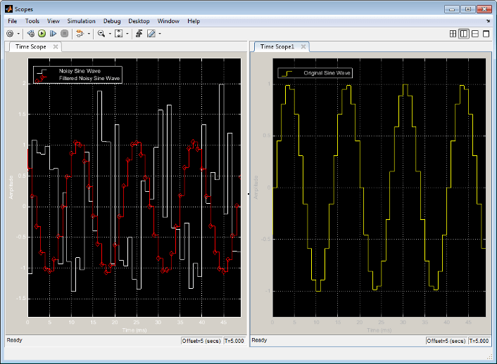
Once docked, the Scopes group container displays the toolbar and menu bar of the Time Scope window. If you open additional instances of Time Scope, a new Time Scope window appears in the Scopes group container.
You can undock any instance of Time Scope by pressing the corresponding Undock
button (![]() ) in the title bar of each docked instance. If
you close the Scopes group container, all docked instances of Time Scope close
but the Simulink model continues to run.
) in the title bar of each docked instance. If
you close the Scopes group container, all docked instances of Time Scope close
but the Simulink model continues to run.
Close All Time Scope Windows
If you save your model with Time Scope windows open, those windows will reopen the next time you open the model. Reopening the Time Scope windows when you open your model can increase the amount of time it takes your model to load. If you are working with a large model, or a model containing multiple Time Scopes, consider closing all Time Scope windows before you save and close that model. To do so, use the File > Close All Time Scope Windows menu option.
To use this menu option in the ex_timescope_tut model, open
the Time Scope or Time Scope1 window, and select File > Close All Time Scope Windows. Both the Time Scope and Time Scope1 windows close. If you now
save and close the model, the Time Scope windows do not automatically open the
next time you open the model. You can open Time Scope windows at any time by
double-clicking a Time Scope block in your model. Alternatively, you can choose
to automatically open the Time Scope windows at simulation start. To do so, from
the Time Scope window, select File > Open at Start of Simulation.
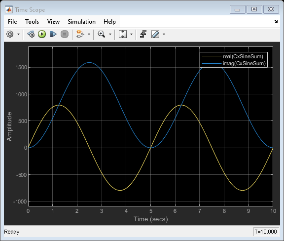
Display Complex-Valued Input Signal
This example shows how to display complex-valued signals in the Time Scope block.
By default, when the input is a complex-valued signal, Time Scope plots the real and imaginary portions on the same axes. These real and imaginary portions appear as different-colored lines on the same axes within the same active display.
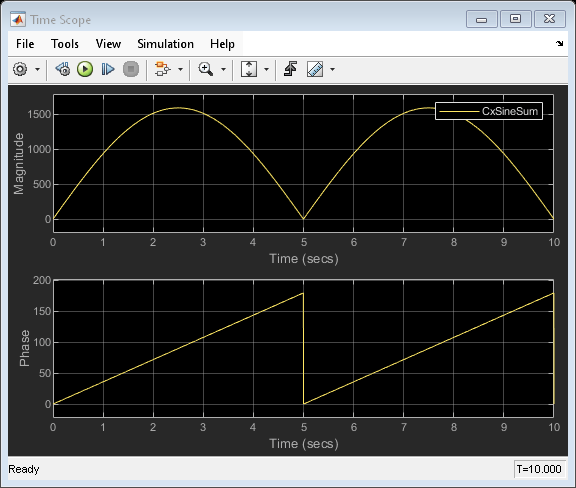
To separate the real and imaginary portions of the input, change the scope to plot magintude and phase.
From the Scope menu, select View > Configuration Properties.
In the Configuration Properties window, on the Display tab, select Plot signal(s) as magnitude and phase.
Click OK. The active display shows the magnitude of the input signal on the top axes. The signal phase, in degrees, appears on the bottom axes.
Display Input Signal of Changing Size
In this example, the size of the input signal to the Time Scope block changes as the simulation progresses.
open_system("ex_timescope_varsize")
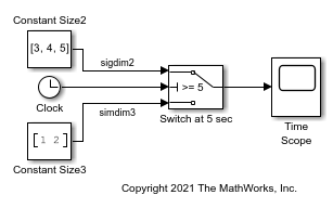
When the simulation time is less than 5 seconds, Time Scope plots the signal connected to the third input port of the Switch block, which has signal dimensions 1 by 2. After 5 seconds, Time Scope plots the signal connected to the first input port of the Switch block, which has signal dimensions 1 by 3.
sim("ex_timescope_varsize")
open_system("ex_timescope_varsize/Time Scope")
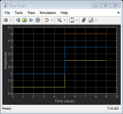
As you can see in the figure, the third line on the display, colored red, appears only after 5 seconds.
Display Simulink Enumeration Input Signal
This example shows how to use the Time Scope to display an enumerated input signal.
open_system("ex_timescope_slenum")
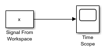
In this example, Simulink® imports the variable x , from the MATLAB® workspace. This variable is created when the model loads because the commands that construct it reside in the model Preload function. To view these commands,
On the Simulink toolbar, on the Modeling tab, in the Setup section, in the drop-down, select
Model Properties.In the Model Properties dialog box, select the
Callbackstab. The following lines of MATLAB® code appear.
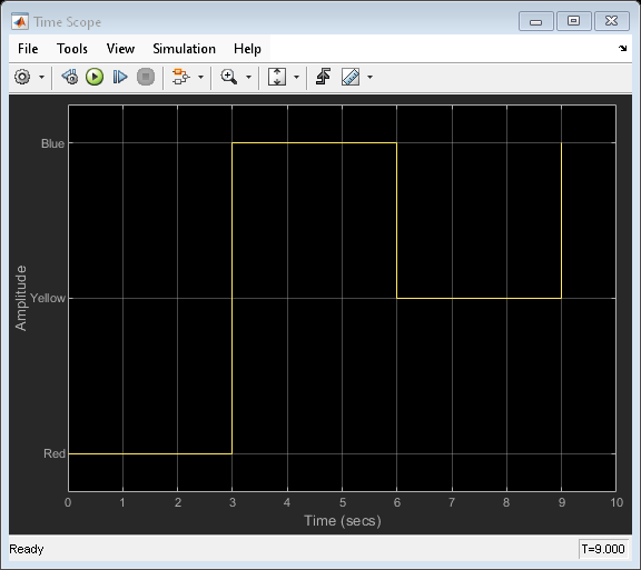
if ~exist('BasicColors','class')
    Simulink.defineIntEnumType('BasicColors', ...
        {'Red', 'Yellow', 'Blue'}, ...
        [0;1;2], ...
        'Description', 'Basic colors', ...
        'DefaultValue', 'Blue', ...
        'AddClassNameToEnumNames', true);
end
x = [BasicColors(0), BasicColors(2), BasicColors(1)]
x =

  1x3 BasicColors enumeration array

    Red       Blue      Yellow
The Signal from Workspace block has a sample time of 3 seconds. Thus, the input signal changes to the next value in vector x every 3 seconds.
sim("ex_timescope_slenum")
open_system("ex_timescope_slenum/Time Scope")
You can also select a web site from the following list:
Americas
- América Latina (Español)
- Canada (English)
- United States (English)
Europe
- Belgium (English)
- Denmark (English)
- Deutschland (Deutsch)
- España (Español)
- Finland (English)
- France (Français)
- Ireland (English)
- Italia (Italiano)
- Luxembourg (English)
- Netherlands (English)
- Norway (English)
- Österreich (Deutsch)
- Portugal (English)
- Sweden (English)
- Switzerland
- United Kingdom (English)