DC Motor Control
This example shows the comparison of three DC motor control techniques for tracking setpoint commands and reducing sensitivity to load disturbances:
feedforward command
integral feedback control
LQR regulation
See "Getting Started: Building Models" for more details about the DC motor model.
Problem Statement
In armature-controlled DC motors, the applied voltage Va controls the angular velocity w of the shaft.
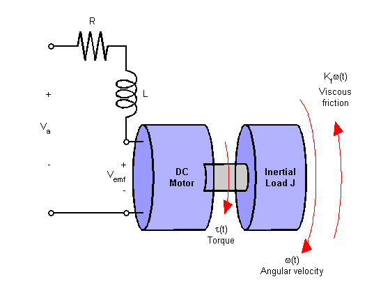
This example shows two DC motor control techniques for reducing the sensitivity of w to load variations (changes in the torque opposed by the motor load).
A simplified model of the DC motor is shown above. The torque Td models load disturbances. You must minimize the speed variations induced by such disturbances.
For this example, the physical constants are:
R = 2.0;                % Ohms
L = 0.5;                % Henrys
Km = 0.1;               % torque constant
Kb = 0.1;               % back emf constant
Kf = 0.2;               % Nms
J = 0.02;               % kg.m^2/s^2
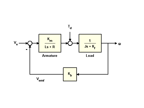
First construct a state-space model of the DC motor with two inputs (Va,Td) and one output (w):
h1 = tf(Km,[L R]);            % armature
h2 = tf(1,[J Kf]);            % eqn of motion

dcm = ss(h2) * [h1 , 1];      % w = h2 * (h1*Va + Td)
dcm = feedback(dcm,Kb,1,1);   % close back emf loop
Note: Compute with the state-space form to minimize the model order.
Now plot the angular velocity response to a step change in voltage Va:
stepplot(dcm(1));
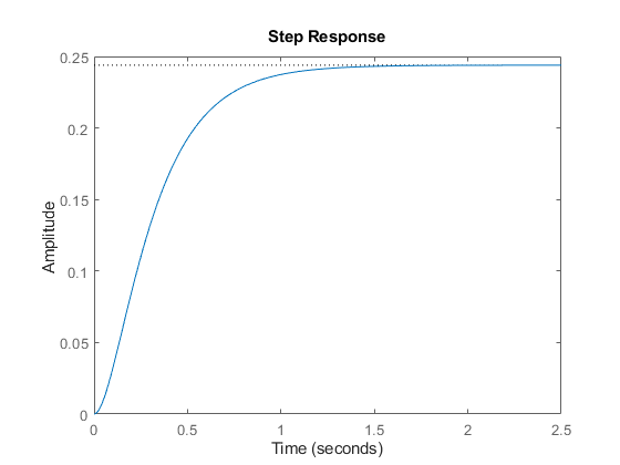
Right-click on the plot and select "Characteristics:Settling Time" to display the settling time.
Feedforward DC Motor Control Design
You can use this simple feedforward control structure to command the angular velocity w to a given value w_ref.
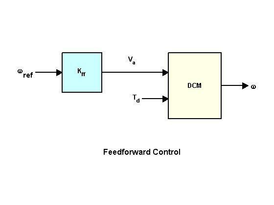
The feedforward gain Kff should be set to the reciprocal of the DC gain from Va to w.
Kff = 1/dcgain(dcm(1))
Kff =

    4.1000
To evaluate the feedforward design in the face of load disturbances, simulate the response to a step command w_ref=1 with a disturbance Td = -0.1Nm between t=5 and t=10 seconds:
t = 0:0.1:15;
Td = -0.1 * (t>5 & t<10);       % load disturbance
u = [ones(size(t)) ; Td];       % w_ref=1 and Td

cl_ff = dcm * diag([Kff,1]);    % add feedforward gain
cl_ff.InputName = {'w_ref','Td'};
cl_ff.OutputName = 'w';

h = lsimplot(cl_ff,u,t);
title('Setpoint tracking and disturbance rejection')
legend('cl\_ff')

% Annotate plot
line([5,5],[.2,.3]);
line([10,10],[.2,.3]);
text(7.5,.25,{'disturbance','T_d = -0.1Nm'},...
            'vertic','middle','horiz','center','color','r');
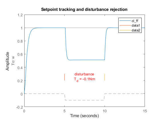
Clearly feedforward control handles load disturbances poorly.
Feedback DC Motor Control Design
Next try the feedback control structure shown below.
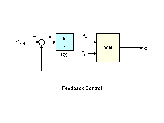
To enforce zero steady-state error, use integral control of the form
C(s) = K/s
where K is to be determined.
To determine the gain K, you can use the root locus technique applied to the open-loop 1/s * transfer(Va->w):
h = rlocusplot(tf(1,[1 0]) * dcm(1));
setoptions(h,'FreqUnits','rad/s');
xlim([-15 5]);
ylim([-15 15]);
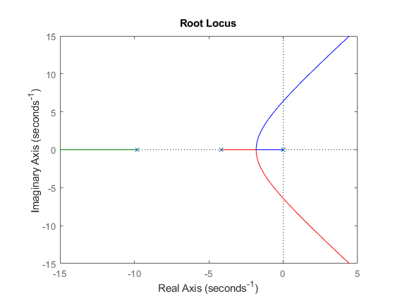
Click on the curves to read the gain values and related info. A reasonable choice here is K = 5. The Control System Designer app is an interactive UI for performing such designs.
Compare this new design with the initial feedforward design on the same test case:
K = 5;
C = tf(K,[1 0]);            % compensator K/s

cl_rloc = feedback(dcm * append(C,1),1,1,1);
h = lsimplot(cl_ff,cl_rloc,u,t);
cl_rloc.InputName = {'w_ref','Td'};
cl_rloc.OutputName = 'w';
title('Setpoint tracking and disturbance rejection')
legend('feedforward','feedback w/ rlocus','Location','NorthWest')
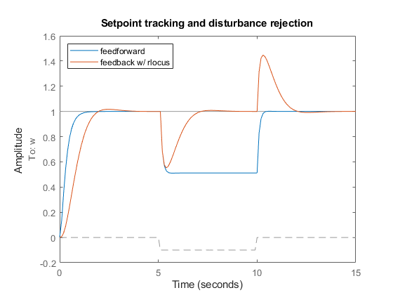
The root locus design is better at rejecting load disturbances.
LQR DC Motor Control Design
To further improve performance, try designing a linear quadratic regulator (LQR) for the feedback structure shown below.
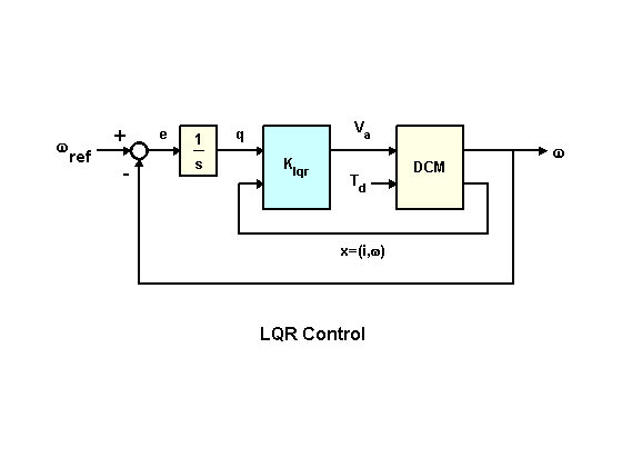
In addition to the integral of error, the LQR scheme also uses the state vector x=(i,w) to synthesize the driving voltage Va. The resulting voltage is of the form
Va = K1 * w + K2 * w/s + K3 * i
where i is the armature current.
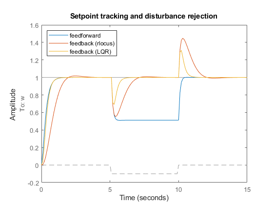
For better disturbance rejection, use a cost function that penalizes large integral error, e.g., the cost function
where

The optimal LQR gain for this cost function is computed as follows:
dc_aug = [1 ; tf(1,[1 0])] * dcm(1); % add output w/s to DC motor model

K_lqr = lqry(dc_aug,[1 0;0 20],0.01);
Next derive the closed-loop model for simulation purposes:
P = augstate(dcm);                     % inputs:Va,Td  outputs:w,x
C = K_lqr * append(tf(1,[1 0]),1,1);   % compensator including 1/s
OL = P * append(C,1);                  % open loop

CL = feedback(OL,eye(3),1:3,1:3);      % close feedback loops
cl_lqr = CL(1,[1 4]);                  % extract transfer (w_ref,Td)->w
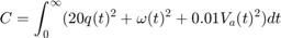
This plot compares the closed-loop Bode diagrams for the three DC motor control designs.
bodeplot(cl_ff,cl_rloc,cl_lqr);
Click on the curves to identify the systems or inspect the data.
Comparison of DC Motor Control Designs
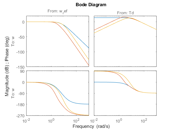
Finally we compare the three DC motor control designs on our simulation test case:
h = lsimplot(cl_ff,cl_rloc,cl_lqr,u,t);
title('Setpoint tracking and disturbance rejection')
legend('feedforward','feedback (rlocus)','feedback (LQR)','Location','NorthWest')
Thanks to its additional degrees of freedom, the LQR compensator performs best at rejecting load disturbances (among the three DC motor control designs discussed here).
You can also select a web site from the following list:
Americas
- América Latina (Español)
- Canada (English)
- United States (English)
Europe
- Belgium (English)
- Denmark (English)
- Deutschland (Deutsch)
- España (Español)
- Finland (English)
- France (Français)
- Ireland (English)
- Italia (Italiano)
- Luxembourg (English)
- Netherlands (English)
- Norway (English)
- Österreich (Deutsch)
- Portugal (English)
- Sweden (English)
- Switzerland
- United Kingdom (English)